

A classification score does not become a probability because it falls between zero and one. Before a workflow uses a score of 0.95 to bypass human review, held-out evidence must show that similarly scored items receive the positive label at about the promised rate.
This article runs that test on an open binary-classification dataset. It keeps training, calibration, and final test rows separate, plots a reliability diagram with bin counts, and measures what happens to an automatic approval lane when the score scale changes. The result shows why threshold selection belongs after calibration testing.
Calibration tests the meaning of the score
A well-calibrated binary classifier gives probabilities that match observed label frequencies. If many examples receive a predicted probability near 0.8, about 80 percent of those examples should belong to the positive class. A reliability diagram checks that relationship by plotting the mean predicted probability in each bin against the observed positive rate in the same bin.
Guo et al. define calibration in the same way for predicted-class confidence. Their experiments found that the tested modern neural networks could be more accurate and less calibrated than older networks. They also found that depth, width, batch normalization, and weight decay affected calibration in the architectures and datasets they studied. Those findings do not prove that every model has the same problem. They show why a model owner must measure the score instead of assuming what it means.
Calibration and ranking answer different questions. ROC AUC is a ranking metric; it does not test whether a score behaves like a probability. Ranking asks whether positive examples tend to receive higher scores than negative examples. Calibration asks whether the score values match observed frequencies. A classifier can rank the rows well while giving probability values that are too close to zero or one.
The scikit-learn calibration guide makes the same separation. It also warns that Brier loss and log loss combine calibration, discrimination, and data uncertainty. They are useful probability-sensitive measures, but neither one proves calibration by itself. The reliability curve and bin counts must remain visible.
Keep training, calibration, and test data separate
The example uses scikit-learn's copy of the Breast Cancer Wisconsin (Diagnostic) dataset, which comes from the UCI Machine Learning Repository. It has 569 rows, 30 numeric features, 212 malignant labels, and 357 benign labels. The features describe cell-nucleus characteristics computed from digitized images of fine-needle aspirates of breast masses.
This is a probability-measurement example, not clinical guidance. The script treats benign as the positive class because scikit-learn encodes it as target 1. The constructed lanes are not a recommendation for diagnosis or medical approval. The automatic, review, and hold lanes demonstrate threshold mechanics only.
The script uses two stratified random splits with random_state=20260803. Stratification preserves the class ratio in each split. The training split has 341 rows, including 214 positive and 127 negative rows. The calibration split has 114 rows, including 71 positive and 43 negative rows. The final test split has 114 rows, including 72 positive and 42 negative rows.
Each split has one job. GaussianNB() fits only the training rows. The sigmoid calibrator fits the base model's outputs and known labels only on the calibration rows. Both score versions are then evaluated on the untouched test rows. If the calibrator fits on the test rows, the final result no longer describes unseen data.
from sklearn.calibration import CalibratedClassifierCV
from sklearn.datasets import load_breast_cancer
from sklearn.frozen import FrozenEstimator
from sklearn.model_selection import train_test_split
from sklearn.naive_bayes import GaussianNB

SEED = 20260803
X, y = load_breast_cancer(return_X_y=True)

X_train, X_remainder, y_train, y_remainder = train_test_split(
    X, y, test_size=0.40, random_state=SEED, stratify=y
)
X_calibration, X_test, y_calibration, y_test = train_test_split(
    X_remainder,
    y_remainder,
    test_size=0.50,
    random_state=SEED,
    stratify=y_remainder,
)

base_model = GaussianNB().fit(X_train, y_train)
calibrated_model = CalibratedClassifierCV(
    estimator=FrozenEstimator(base_model),
    method="sigmoid",
).fit(X_calibration, y_calibration)
scikit-learn documents FrozenEstimator for an already fitted classifier and puts responsibility for the data separation on the user. The example uses sigmoid calibration because the calibration split is small and the method preserves score ranking. The documentation warns that isotonic calibration is more prone to overfitting on small datasets and generally needs more than about 1,000 calibration examples.
Download the complete, versioned evidence package:
Run the script with:
uv run --with-requirements requirements.txt python calibration_example.py
The verified run used Python 3.11.15, NumPy 2.4.6, SciPy 1.17.1, Matplotlib 3.11.1, and scikit-learn 1.9.0. It writes the full metrics to JSON, every reliability bin to CSV, and the chart as PNG and SVG.
The bin counts control what the curve can support
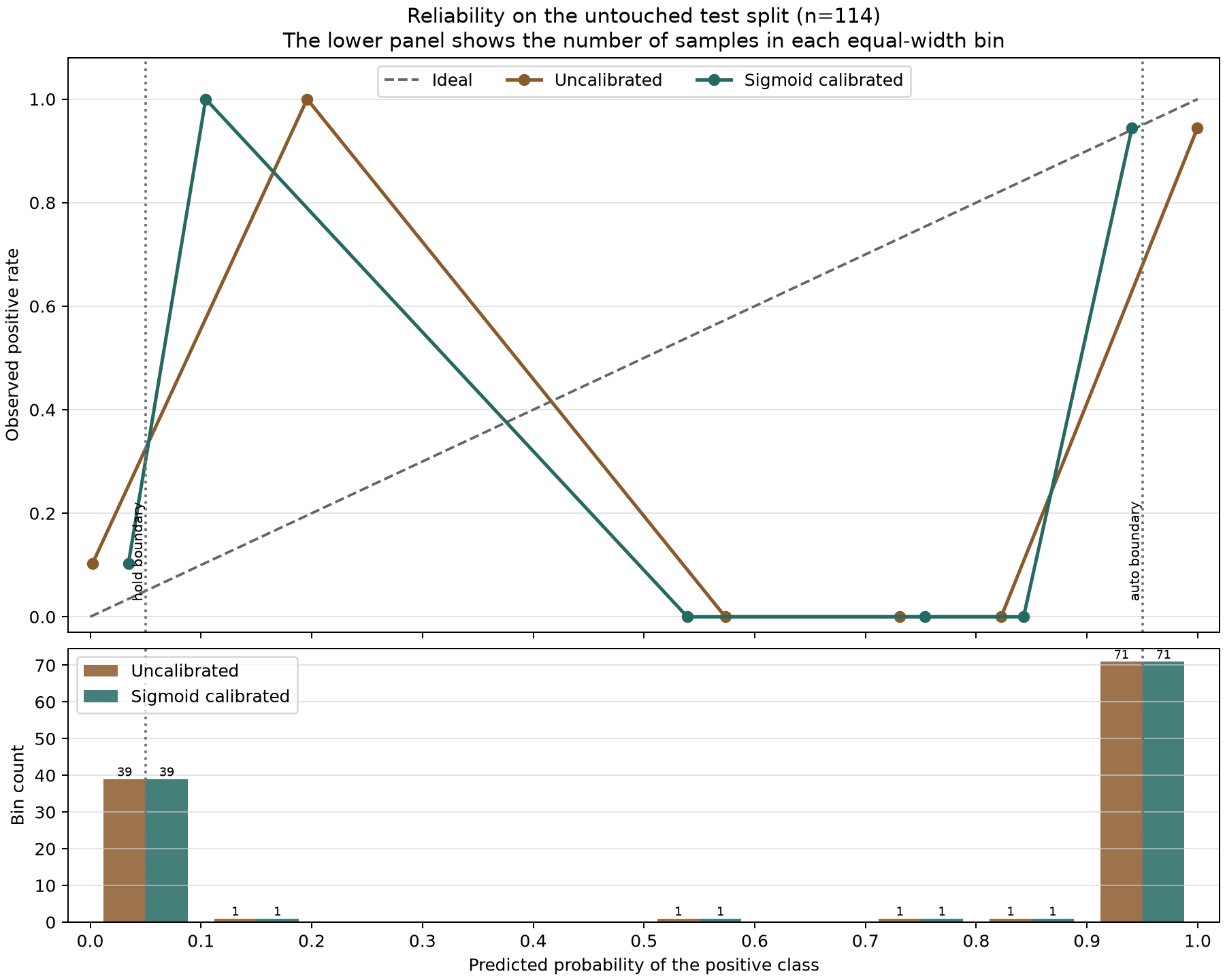
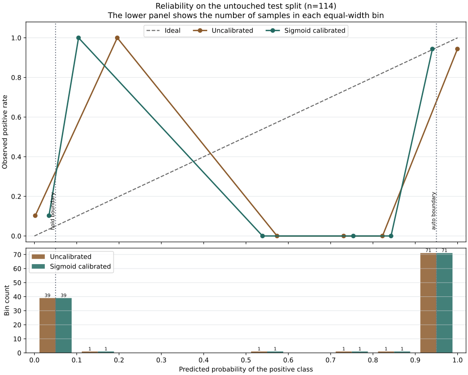
The reliability diagram uses ten equal-width probability bins. Its upper panel plots the observed positive rate against the mean predicted probability for each nonempty bin. The lower panel shows the number of test rows in every bin.
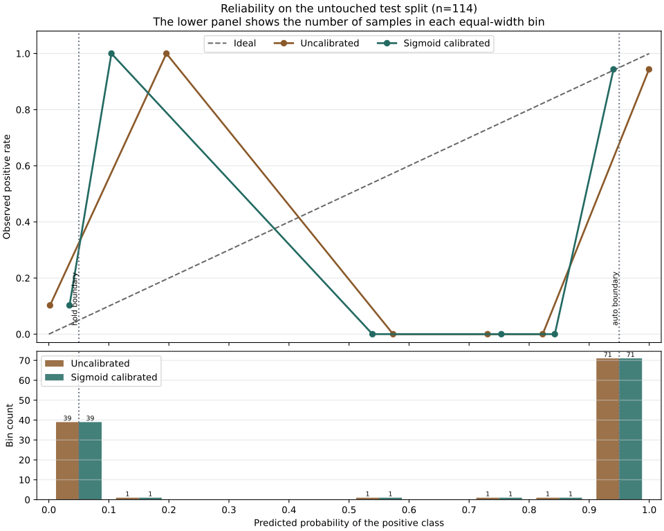
Most test rows sit in the extreme bins. Sigmoid calibration moves the high-bin mean from 0.999660 to 0.940526 while its observed positive rate remains 0.943662. One-row middle bins remain weak evidence. Open the full-size SVG or download every bin value as CSV.
Scroll sideways to see all 3 columns.
| Probability bin | Uncalibrated count | Sigmoid-calibrated count |
|---|---|---|
| 0.0–0.1 | 39 | 39 |
| 0.1–0.2 | 1 | 1 |
| 0.2–0.3 | 0 | 0 |
| 0.3–0.4 | 0 | 0 |
| 0.4–0.5 | 0 | 0 |
| 0.5–0.6 | 1 | 1 |
| 0.6–0.7 | 0 | 0 |
| 0.7–0.8 | 1 | 1 |
| 0.8–0.9 | 1 | 1 |
| 0.9–1.0 | 71 | 71 |
The raw classifier placed 39 rows in the 0.0–0.1 bin. Their mean predicted probability was 0.002011, but their observed positive rate was 0.102564. It also placed 71 rows in the 0.9–1.0 bin. Their mean predicted probability was 0.999660, while their observed positive rate was 0.943662. The raw scores were more extreme than the held-out labels supported.
After sigmoid calibration, the 0.0–0.1 bin also contained 39 rows and had a mean probability of 0.034478. The 0.9–1.0 bin also contained 71 rows and had a mean probability of 0.940526, close to its observed positive rate of 0.943662. The transformation changed the probability values without changing the row order.
The middle of the curve is weak evidence. Every occupied middle bin contains one row, and four middle bins are empty. A point at zero or one from one row is not a stable probability estimate. The count panel prevents the line from looking more certain than the sample permits.
Ranking stayed the same while probability measures changed
The untouched test split produced these results:
Scroll sideways to see all 5 columns.
| Score version | ROC AUC | Brier loss | Log loss | ECE, 10 bins |
|---|---|---|---|---|
| Uncalibrated | 0.973545 | 0.089369 | 1.355334 | 0.094987 |
| Sigmoid calibrated | 0.973545 | 0.087027 | 0.319629 | 0.051836 |
ROC AUC stayed at 0.973545 because sigmoid calibration is a strictly monotonic transformation. The classifier ranked the rows in the same order. The test did not make the base classifier better at ranking benign above malignant examples.
The probability-sensitive measures changed. Brier loss fell by 0.002342, log loss fell by 1.035705, and ten-bin expected calibration error fell by 0.043151. The large log-loss change reflects how strongly log loss penalizes confident wrong probabilities. These values support a narrower claim: sigmoid calibration improved the reported probability behavior on this test split.
They do not establish that the calibrated model is ready for an automatic decision. Brier loss and log loss include more than calibration. Expected calibration error changes with the bins and sample. The middle bins are sparse, and the test has only 114 rows.
The same 0.95 threshold created a different queue
To make the operational consequence visible, the script applies one constructed policy to both score versions. It auto-approves the positive-class classification at 0.95 or higher, sends scores from 0.05 through 0.95 to manual review, and holds scores below 0.05.
Scroll sideways to see all 3 columns.
| Consequence on 114 test rows | Uncalibrated | Sigmoid calibrated |
|---|---|---|
| Automatic lane | 71 | 0 |
| Manual-review lane | 5 | 76 |
| Hold lane | 38 | 38 |
| Review share | 4.4% | 66.7% |
| Negative rows in the automatic lane | 4 | 0 |
| Positive rows in the hold lane | 4 | 4 |
The raw score would have sent 71 rows through the automatic lane, including four negative rows. The calibrated score sent none through the same 0.95 boundary. In total, 71 rows moved from automatic handling into manual review, which increased the review share from 4.4 percent to 66.7 percent.
This change did not correct the four rows or teach the classifier a new order. Calibration changed the score scale without improving ranking, and the fixed policy acted on that new scale. It did not repair labels, remove classification errors, or make the workflow safe for production. That is why reviewer capacity and error consequences must be recalculated after calibration and before approval thresholds go live.
The constructed 0.95 policy does not have enough evidence for an automatic lane. The high bin's observed positive rate was 94.4 percent, and it contained four negative rows. Lowering the threshold to restore the prior queue size would reverse the order of work. The team would be choosing a convenient review volume first and assigning probability meaning afterward.
Use threshold tuning for AI approval workflows after the probability test supports the score scale. Use precision and recall to compare false automatic approvals with safe work that remains in review or hold. Keep the score-policy boundary explicit because a calibrated probability still does not include consequence, reversibility, missing evidence, or a prohibited action.
Calibration does not repair the data or the workflow
Calibration is a fitted mapping from model output to observed label frequency under the sampled conditions. It does not fix distribution shift, poor labels, a missing class, weak features, a weak classifier, or a future population that differs from the calibration and test data. It also does not decide whether the positive class is the right business target.
A deployed workflow needs a representative time boundary, class and subgroup coverage, stable label definitions, and a plan to repeat the test. Reviewers need to see the score version, policy rule, source evidence, and missing information for each item. The AI workflow controls guide connects that review to permissions, monitoring, escalation, and rollback.
The AI agent receipt template gives each run a place to record the score, routing lane, model version, policy boundary, reviewer decision, final action, and correction path. Store enough detail to reconstruct which calibration version and threshold controlled the item. A later calibration change should not turn old decisions into unexplained records.
For this sample, the next action is to keep automatic handling closed. Collect a larger representative calibration and test set, define the acceptable false-approval cost and reviewer capacity, and rerun the reliability and queue analysis. If your team needs help connecting those steps, BaristaLabs can review one model score through its AI consulting service.
For this sample, the next action is to keep automatic handling closed. Collect a larger representative calibration and test set, define the acceptable false-approval cost and reviewer capacity, and rerun the reliability and queue analysis.
Source note
Guo et al. control the calibration definition, reliability-diagram and equal-width expected-calibration-error method, and the paper's findings about its tested neural-network architectures, datasets, and temperature-scaling experiments. scikit-learn controls CalibratedClassifierCV, FrozenEstimator, sigmoid and isotonic behavior, calibration-curve semantics, the bin-count guidance, and the Brier- and log-loss caveat.
The split, Gaussian Naive Bayes classifier, sigmoid fit, ten-bin results, workflow thresholds, lane counts, code, plot, operational interpretation, and recommendation to keep this constructed automatic lane closed are BaristaLabs teaching material from the executed example. The dataset does not support medical use or a production performance claim.
Calibration review
Test the score before it controls the queue
BaristaLabs can help your team separate training, calibration, and test data, read the reliability evidence, and connect a supported threshold to reviewer capacity and error costs.
Best fit when a workflow already produces classification scores and the team is deciding which items may bypass review.
Calibration review
Test the score before it controls the queue
Bring one scored workflow. BaristaLabs can help you separate training, calibration, and test data, then connect the threshold to reviewer capacity and error costs.
Review one model scoreBest fit when a workflow already produces scores and the team must decide which items can bypass review.
Turn this idea into a pilot
Which workflow should go first?
Use the readiness check to compare impact, effort, risk, owner, and next step before requesting a review.
- 3-5 minutes
- Deterministic score
- No sensitive data
Practical AI Workflow Notes
Want more practical AI operations ideas?
Get short notes on applying AI inside real small-business workflows — from document handling and customer follow-up to internal reporting, compliance, and automation guardrails.