


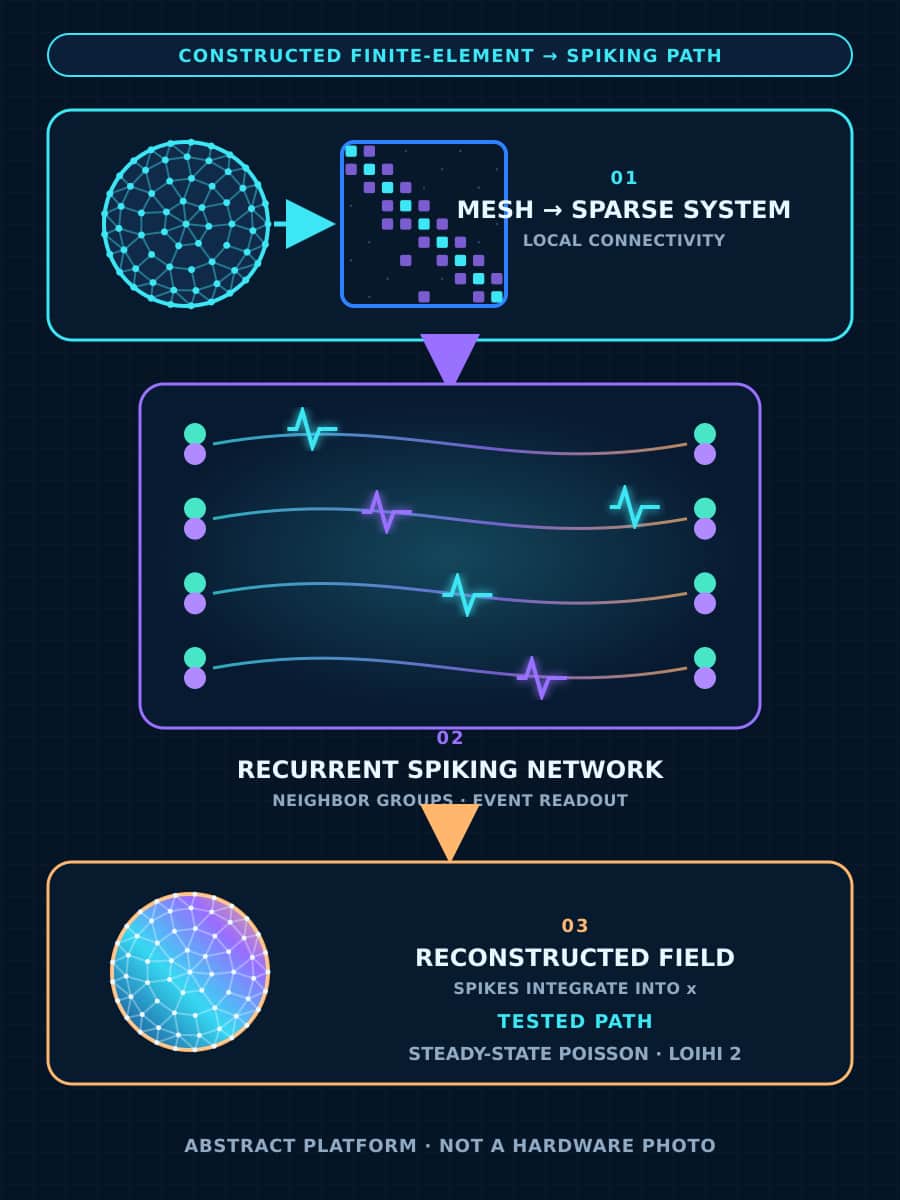
Sandia researchers mapped the linear-system solve inside the finite element method to Intel's Loihi 2. The finite element method (FEM) is a numerical method that divides a physical domain into a mesh of small elements, then approximates a solution across that mesh. Loihi 2 is Intel's digital neuromorphic chip for running sparse networks of artificial neurons with asynchronous spike events.
The paper in Nature Machine Intelligence focuses on sparse linear systems: sets of equations whose matrices contain mostly zero entries because each mesh point connects to only nearby points. The researchers built a recurrent spiking neural network (SNN), a network that communicates through timed spike events, to solve those systems. This creates a working finite-element solver on neuromorphic hardware and gives the paper measured accuracy and scaling results. General production parity and a universal energy advantage remain unestablished.
A finite-element mesh becomes a sparse linear system
A partial differential equation (PDE) describes how a quantity changes across space, time, or both. Engineers use PDEs to model heat, stress, fields, fluids, and other physical behavior. The finite element method makes a PDE computable by dividing its domain into a mesh and approximating the solution with functions attached to the mesh elements.
That process produces a linear system often written as Ax = b. The matrix A records how the mesh points interact, b contains the applied input or forcing function, and x contains the coefficients that approximate the PDE solution. Most entries in A are zero because a mesh point usually interacts with its nearest neighbors. This sparsity is useful, but it also makes data movement and memory bandwidth important costs for conventional large-scale solvers.
The local structure gives neuromorphic hardware a plausible fit. A mesh node can connect to a small neuron population, and the network can send discrete spike events only along the connections that exist. The paper tests whether those local dynamics can move the network toward the same linear-system solution that a conventional finite-element workflow needs.
The spiking network is programmed from the finite-element system
The authors interpret Ax = b as a dynamical system whose state moves toward the solution. Each mesh node receives a small population of recurrently connected neurons. Values from A determine synaptic weights between populations, and values from b become input biases. A readout integrates the spikes from each population into an estimate of the corresponding value in x.
The first direct mapping left a steady-state error. The researchers corrected it by adding a local integral of the residual error to each neuron. This turns the neurons into distributed proportional-integral controllers and removes the steady-state bias while keeping communication local.
The mapping does not require model training. The weights, biases, and neuron dynamics come from the finite-element system. After the network is built for a given equation, boundary condition, mesh, and finite-element space, it can accept a new right-hand side by changing the biases. The paper demonstrates this reconfiguration in simulation without retraining the network.
The accuracy result is bounded to the tested problems and settings
The main benchmark is the steady-state Poisson equation on a disk with fixed boundary values and a known analytic solution. In floating-point CPU simulations, the authors tested meshes with approximately 100 to 10,000 nodes. They averaged the spiking readout over 10,000 timesteps after the network reached steady state, then compared it with the analytic solution and SciPy's conventional spsolve result.
For that benchmark, the spiking solver produced comparably accurate solutions as mesh resolution increased. It also showed the same quadratic finite-element convergence expected from the piecewise-linear elements. The paper reports an important limit beside that result: the absolute linear-system residual was worse than the residual from spsolve, and accuracy depended on network parameters and the number of samples averaged.
The hardware test was narrower. On one Loihi 2 chip, the authors ran Poisson meshes with 103 to 967 nodes. Fixed-point conversion added numerical error. The paper's Figure 3 reports about 4% average relative deviation from the conventional solution across mesh nodes, with a maximum of approximately 8%. Configurations with 16 neurons per mesh node did not reliably converge below approximately 200 mesh nodes, while the larger tested networks converged.
These results support meaningful numerical accuracy for the reported Poisson setup. They do not support a claim that Loihi 2 matched conventional solvers across finite-element workloads.

The energy measurement excludes input, output, and a full CPU energy benchmark
For its single-chip profiling, the study used Poisson meshes of approximately 100 to 1,000 nodes. The researchers disabled hardware input and output. They changed the right-hand side every 4,096 timesteps, measured the transient that moved the network to a new solution, and subtracted the energy and time of a network that stayed at steady state.
Under that measurement, the additional energy was at most approximately 80 millijoules per solution epoch for the tested meshes. The transient case required at most about 30 milliseconds more per epoch than the steady-state case. The paper also says the same system solved faster on a CPU: approximately 1 to 2 times faster with the generalized minimum residual method and approximately 10 to 20 times faster with conjugate gradient. The authors estimate that Loihi 2 used less energy, but they state that optimized CPU profiling is mesh-dependent and outside the study's scope.
The result is a bounded on-chip energy estimate for one Poisson setup. It excludes hardware input and output, and it does not provide a complete end-to-end energy comparison that includes host work, data transfer, preprocessing, or an optimized conventional baseline.
The scaling result is stronger within its own boundary. Across the full 32-chip Loihi 2 platform, NeuroFEM showed close-to-ideal strong scaling over a limited range for fixed-size problems. It also showed near-ideal weak scaling for a fixed number of mesh points per core until overhead and hardware limits reduced the gains. This measures the parallel efficiency of NeuroFEM as resources and problem size increase. It does not show general speed superiority over an optimized CPU solver.
The irregular-mesh and elasticity examples ran in CPU simulation
The authors also tested whether the formulation extends beyond the disk benchmark. In CPU simulation, NeuroFEM solved the Poisson equation on an irregular two-dimensional domain with holes, mixed boundary conditions, and nonuniform mesh resolution. A second CPU example solved static linear elasticity on an irregular three-dimensional tetrahedral mesh and produced a displacement field close to the conventional result.
These examples show that the mapping can represent more complex mesh geometry and a system of elasticity equations. The paper does not report those broader examples as Loihi 2 hardware runs. They support an algorithmic extension, not hardware validation for general production PDE workloads.
The paper leaves production economics and downstream outcomes open
The paper demonstrates one direct path from established finite-element mathematics to spiking hardware. It does not test the range of nonlinear, time-dependent, coupled, ill-conditioned, or adaptively meshed systems that a production scientific-computing program can contain. It also does not compare NeuroFEM with optimized conventional solvers across representative workloads, precisions, preconditioners, convergence targets, and hardware configurations.
The energy boundary remains equally important. The paper isolates transient work on Loihi 2 with input and output disabled. A production claim needs the energy and time for the complete path, including data preparation, host coordination, transfer, output, repeated runs, and cooling or shared-system overhead where those costs apply. The baseline must use an optimized solver that meets the same numerical acceptance criteria.
The official Sandia release describes possible neuromorphic supercomputers, national-security uses, and medical insight. Those are future directions in the release. The paper does not report a deployed neuromorphic supercomputer, production national-security simulations, medical outcomes, or evidence that the brain directly solves PDEs with this method. In fact, the paper says it is unlikely that the cortex solves PDEs directly in this way.
A production evaluation must preserve the workload and measurement boundary
BaristaLabs recommends treating the paper as a candidate architecture result, then building a direct comparison around one real workload. The evaluation should record:
- The exact PDE, sparse system, mesh sizes, boundary conditions, and production input distribution, along with the current optimized solver and hardware baseline.
- Required precision, error and residual measures, convergence threshold, condition-number range, stop rule, and result tolerance.
- Chip, core, memory, and interconnect utilization, including partitioning, saturation, latency, throughput, and failed or unstable runs.
- The full energy boundary, with host work, input and output, data movement, preprocessing, idle power, repeated runs, and any excluded costs stated separately.
- Code, compiler, microcode, parameter, and hardware versions; run counts; variance; reproducible inputs; and an owner for the evidence. The paper makes its CPU simulation code public, while its Loihi 2-specific code is proprietary.
- Availability, maintenance, total cost, failure detection, and the tested fallback when the specialized path does not converge or is unavailable.
The production AI model evaluation guide provides a record for comparing one candidate with the current path under the same acceptance bar. If the experiment becomes a production dependency, the Model Facts Register can keep the exact hardware and software path, owner, review trigger, and fallback visible.
The paper earns attention because it maps an established numerical method directly to neuromorphic hardware and tests the result. Its production economics remain open. The next decision should come from a workload-matched benchmark with an optimized baseline and a complete energy boundary.
Sources
- Bradley H. Theilman and James B. Aimone, "Solving sparse finite element problems on neuromorphic hardware", Nature Machine Intelligence 7, 1845–1857 (2025), published November 13, 2025. This version-of-record paper is the primary evidence source.
- Nature publisher page and open-access full text, including the methods, figures, extended data, supplementary files, data-availability statement, and code-availability statement.
- Sandia National Laboratories, "Nature-inspired computers are shockingly good at math", published January 7, 2026. This official release is used only for release context and future-direction claims.
- Sandia's NeuroFEM repository, which the paper identifies as the public implementation of the CPU simulations. The paper says the Loihi 2-specific code is proprietary.
- ScienceDaily reproduction of the Sandia release. It is not the official announcement and is not used here as evidence for the research result.